July 1, 2022

Welcome to the wonderful world of widgets.

Today's widget is a predictive neural network.

STEPS

  1. Import Dependancies & Load Dataset
  2. Pre-process Data
    a) check the dataset for unwanted columns, missing values, data type
    b) separate target column from features columns
  3. Split dataset into training and test data, then standarize data
  4. Build Neural Network
    a) keras layers
    b) complie by data type
  5. Train Neural Network
  6. Visualize Performance and Probabilities
    a) accuracy plot
    b) loss plot
    c) probability indices
  7. Build Predictive System

Predictive System Output
1: benign
0: malignant
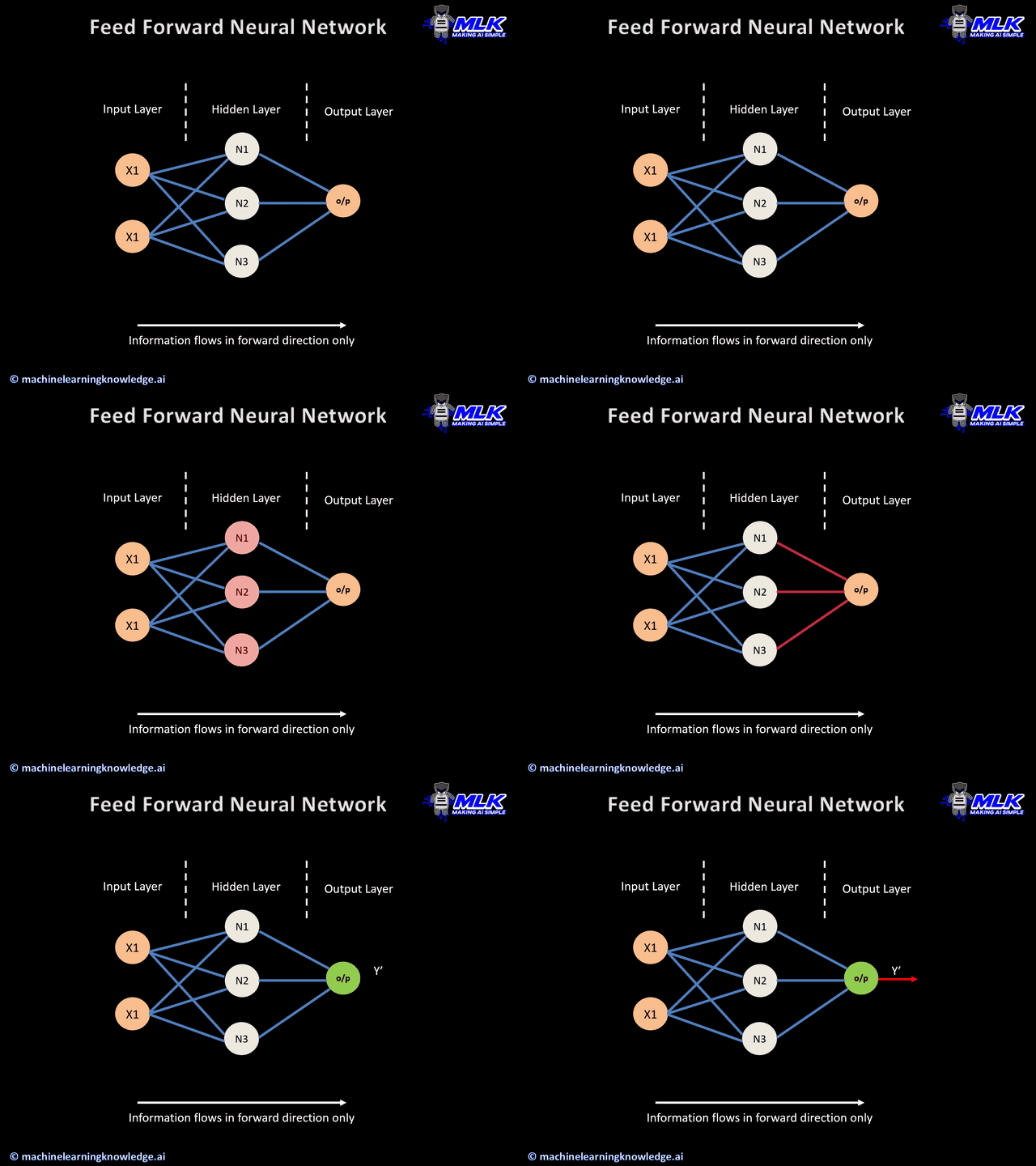
https://machinelearningknowledge.ai/wp-content/uploads/2019/10/Feed-Forward-Neural-Network.gif
In [74]:
# https://www.youtube.com/watch?v=WGNI-k20GNo

#data array
import numpy as np

#data frame
import pandas as pd

#data collection, load breast cancer dataset from sklearn to pandas data frame
import sklearn.datasets
data = sklearn.datasets.load_breast_cancer()

from sklearn.model_selection import train_test_split
from sklearn.linear_model import LogisticRegression
from sklearn.metrics import accuracy_score

Dataset Processing

In [75]:
print(data)
{'data': array([[1.799e+01, 1.038e+01, 1.228e+02, ..., 2.654e-01, 4.601e-01,
        1.189e-01],
       [2.057e+01, 1.777e+01, 1.329e+02, ..., 1.860e-01, 2.750e-01,
        8.902e-02],
       [1.969e+01, 2.125e+01, 1.300e+02, ..., 2.430e-01, 3.613e-01,
        8.758e-02],
       ...,
       [1.660e+01, 2.808e+01, 1.083e+02, ..., 1.418e-01, 2.218e-01,
        7.820e-02],
       [2.060e+01, 2.933e+01, 1.401e+02, ..., 2.650e-01, 4.087e-01,
        1.240e-01],
       [7.760e+00, 2.454e+01, 4.792e+01, ..., 0.000e+00, 2.871e-01,
        7.039e-02]]), 'target': array([0, 0, 0, 0, 0, 0, 0, 0, 0, 0, 0, 0, 0, 0, 0, 0, 0, 0, 0, 1, 1, 1,
       0, 0, 0, 0, 0, 0, 0, 0, 0, 0, 0, 0, 0, 0, 0, 1, 0, 0, 0, 0, 0, 0,
       0, 0, 1, 0, 1, 1, 1, 1, 1, 0, 0, 1, 0, 0, 1, 1, 1, 1, 0, 1, 0, 0,
       1, 1, 1, 1, 0, 1, 0, 0, 1, 0, 1, 0, 0, 1, 1, 1, 0, 0, 1, 0, 0, 0,
       1, 1, 1, 0, 1, 1, 0, 0, 1, 1, 1, 0, 0, 1, 1, 1, 1, 0, 1, 1, 0, 1,
       1, 1, 1, 1, 1, 1, 1, 0, 0, 0, 1, 0, 0, 1, 1, 1, 0, 0, 1, 0, 1, 0,
       0, 1, 0, 0, 1, 1, 0, 1, 1, 0, 1, 1, 1, 1, 0, 1, 1, 1, 1, 1, 1, 1,
       1, 1, 0, 1, 1, 1, 1, 0, 0, 1, 0, 1, 1, 0, 0, 1, 1, 0, 0, 1, 1, 1,
       1, 0, 1, 1, 0, 0, 0, 1, 0, 1, 0, 1, 1, 1, 0, 1, 1, 0, 0, 1, 0, 0,
       0, 0, 1, 0, 0, 0, 1, 0, 1, 0, 1, 1, 0, 1, 0, 0, 0, 0, 1, 1, 0, 0,
       1, 1, 1, 0, 1, 1, 1, 1, 1, 0, 0, 1, 1, 0, 1, 1, 0, 0, 1, 0, 1, 1,
       1, 1, 0, 1, 1, 1, 1, 1, 0, 1, 0, 0, 0, 0, 0, 0, 0, 0, 0, 0, 0, 0,
       0, 0, 1, 1, 1, 1, 1, 1, 0, 1, 0, 1, 1, 0, 1, 1, 0, 1, 0, 0, 1, 1,
       1, 1, 1, 1, 1, 1, 1, 1, 1, 1, 1, 0, 1, 1, 0, 1, 0, 1, 1, 1, 1, 1,
       1, 1, 1, 1, 1, 1, 1, 1, 1, 0, 1, 1, 1, 0, 1, 0, 1, 1, 1, 1, 0, 0,
       0, 1, 1, 1, 1, 0, 1, 0, 1, 0, 1, 1, 1, 0, 1, 1, 1, 1, 1, 1, 1, 0,
       0, 0, 1, 1, 1, 1, 1, 1, 1, 1, 1, 1, 1, 0, 0, 1, 0, 0, 0, 1, 0, 0,
       1, 1, 1, 1, 1, 0, 1, 1, 1, 1, 1, 0, 1, 1, 1, 0, 1, 1, 0, 0, 1, 1,
       1, 1, 1, 1, 0, 1, 1, 1, 1, 1, 1, 1, 0, 1, 1, 1, 1, 1, 0, 1, 1, 0,
       1, 1, 1, 1, 1, 1, 1, 1, 1, 1, 1, 1, 0, 1, 0, 0, 1, 0, 1, 1, 1, 1,
       1, 0, 1, 1, 0, 1, 0, 1, 1, 0, 1, 0, 1, 1, 1, 1, 1, 1, 1, 1, 0, 0,
       1, 1, 1, 1, 1, 1, 0, 1, 1, 1, 1, 1, 1, 1, 1, 1, 1, 0, 1, 1, 1, 1,
       1, 1, 1, 0, 1, 0, 1, 1, 0, 1, 1, 1, 1, 1, 0, 0, 1, 0, 1, 0, 1, 1,
       1, 1, 1, 0, 1, 1, 0, 1, 0, 1, 0, 0, 1, 1, 1, 0, 1, 1, 1, 1, 1, 1,
       1, 1, 1, 1, 1, 0, 1, 0, 0, 1, 1, 1, 1, 1, 1, 1, 1, 1, 1, 1, 1, 1,
       1, 1, 1, 1, 1, 1, 1, 1, 1, 1, 1, 1, 0, 0, 0, 0, 0, 0, 1]), 'frame': None, 'target_names': array(['malignant', 'benign'], dtype='<U9'), 'DESCR': '.. _breast_cancer_dataset:\n\nBreast cancer wisconsin (diagnostic) dataset\n--------------------------------------------\n\n**Data Set Characteristics:**\n\n    :Number of Instances: 569\n\n    :Number of Attributes: 30 numeric, predictive attributes and the class\n\n    :Attribute Information:\n        - radius (mean of distances from center to points on the perimeter)\n        - texture (standard deviation of gray-scale values)\n        - perimeter\n        - area\n        - smoothness (local variation in radius lengths)\n        - compactness (perimeter^2 / area - 1.0)\n        - concavity (severity of concave portions of the contour)\n        - concave points (number of concave portions of the contour)\n        - symmetry\n        - fractal dimension ("coastline approximation" - 1)\n\n        The mean, standard error, and "worst" or largest (mean of the three\n        worst/largest values) of these features were computed for each image,\n        resulting in 30 features.  For instance, field 0 is Mean Radius, field\n        10 is Radius SE, field 20 is Worst Radius.\n\n        - class:\n                - WDBC-Malignant\n                - WDBC-Benign\n\n    :Summary Statistics:\n\n    ===================================== ====== ======\n                                           Min    Max\n    ===================================== ====== ======\n    radius (mean):                        6.981  28.11\n    texture (mean):                       9.71   39.28\n    perimeter (mean):                     43.79  188.5\n    area (mean):                          143.5  2501.0\n    smoothness (mean):                    0.053  0.163\n    compactness (mean):                   0.019  0.345\n    concavity (mean):                     0.0    0.427\n    concave points (mean):                0.0    0.201\n    symmetry (mean):                      0.106  0.304\n    fractal dimension (mean):             0.05   0.097\n    radius (standard error):              0.112  2.873\n    texture (standard error):             0.36   4.885\n    perimeter (standard error):           0.757  21.98\n    area (standard error):                6.802  542.2\n    smoothness (standard error):          0.002  0.031\n    compactness (standard error):         0.002  0.135\n    concavity (standard error):           0.0    0.396\n    concave points (standard error):      0.0    0.053\n    symmetry (standard error):            0.008  0.079\n    fractal dimension (standard error):   0.001  0.03\n    radius (worst):                       7.93   36.04\n    texture (worst):                      12.02  49.54\n    perimeter (worst):                    50.41  251.2\n    area (worst):                         185.2  4254.0\n    smoothness (worst):                   0.071  0.223\n    compactness (worst):                  0.027  1.058\n    concavity (worst):                    0.0    1.252\n    concave points (worst):               0.0    0.291\n    symmetry (worst):                     0.156  0.664\n    fractal dimension (worst):            0.055  0.208\n    ===================================== ====== ======\n\n    :Missing Attribute Values: None\n\n    :Class Distribution: 212 - Malignant, 357 - Benign\n\n    :Creator:  Dr. William H. Wolberg, W. Nick Street, Olvi L. Mangasarian\n\n    :Donor: Nick Street\n\n    :Date: November, 1995\n\nThis is a copy of UCI ML Breast Cancer Wisconsin (Diagnostic) datasets.\nhttps://goo.gl/U2Uwz2\n\nFeatures are computed from a digitized image of a fine needle\naspirate (FNA) of a breast mass.  They describe\ncharacteristics of the cell nuclei present in the image.\n\nSeparating plane described above was obtained using\nMultisurface Method-Tree (MSM-T) [K. P. Bennett, "Decision Tree\nConstruction Via Linear Programming." Proceedings of the 4th\nMidwest Artificial Intelligence and Cognitive Science Society,\npp. 97-101, 1992], a classification method which uses linear\nprogramming to construct a decision tree.  Relevant features\nwere selected using an exhaustive search in the space of 1-4\nfeatures and 1-3 separating planes.\n\nThe actual linear program used to obtain the separating plane\nin the 3-dimensional space is that described in:\n[K. P. Bennett and O. L. Mangasarian: "Robust Linear\nProgramming Discrimination of Two Linearly Inseparable Sets",\nOptimization Methods and Software 1, 1992, 23-34].\n\nThis database is also available through the UW CS ftp server:\n\nftp ftp.cs.wisc.edu\ncd math-prog/cpo-dataset/machine-learn/WDBC/\n\n.. topic:: References\n\n   - W.N. Street, W.H. Wolberg and O.L. Mangasarian. Nuclear feature extraction \n     for breast tumor diagnosis. IS&T/SPIE 1993 International Symposium on \n     Electronic Imaging: Science and Technology, volume 1905, pages 861-870,\n     San Jose, CA, 1993.\n   - O.L. Mangasarian, W.N. Street and W.H. Wolberg. Breast cancer diagnosis and \n     prognosis via linear programming. Operations Research, 43(4), pages 570-577, \n     July-August 1995.\n   - W.H. Wolberg, W.N. Street, and O.L. Mangasarian. Machine learning techniques\n     to diagnose breast cancer from fine-needle aspirates. Cancer Letters 77 (1994) \n     163-171.', 'feature_names': array(['mean radius', 'mean texture', 'mean perimeter', 'mean area',
       'mean smoothness', 'mean compactness', 'mean concavity',
       'mean concave points', 'mean symmetry', 'mean fractal dimension',
       'radius error', 'texture error', 'perimeter error', 'area error',
       'smoothness error', 'compactness error', 'concavity error',
       'concave points error', 'symmetry error',
       'fractal dimension error', 'worst radius', 'worst texture',
       'worst perimeter', 'worst area', 'worst smoothness',
       'worst compactness', 'worst concavity', 'worst concave points',
       'worst symmetry', 'worst fractal dimension'], dtype='<U23'), 'filename': 'breast_cancer.csv', 'data_module': 'sklearn.datasets.data'}
In [76]:
#load data into data frame
data_frame = pd.DataFrame(data.data, columns = data.feature_names)

#print last 5 rows
data_frame.tail()
Out[76]:
mean radius mean texture mean perimeter mean area mean smoothness mean compactness mean concavity mean concave points mean symmetry mean fractal dimension ... worst radius worst texture worst perimeter worst area worst smoothness worst compactness worst concavity worst concave points worst symmetry worst fractal dimension
564 21.56 22.39 142.00 1479.0 0.11100 0.11590 0.24390 0.13890 0.1726 0.05623 ... 25.450 26.40 166.10 2027.0 0.14100 0.21130 0.4107 0.2216 0.2060 0.07115
565 20.13 28.25 131.20 1261.0 0.09780 0.10340 0.14400 0.09791 0.1752 0.05533 ... 23.690 38.25 155.00 1731.0 0.11660 0.19220 0.3215 0.1628 0.2572 0.06637
566 16.60 28.08 108.30 858.1 0.08455 0.10230 0.09251 0.05302 0.1590 0.05648 ... 18.980 34.12 126.70 1124.0 0.11390 0.30940 0.3403 0.1418 0.2218 0.07820
567 20.60 29.33 140.10 1265.0 0.11780 0.27700 0.35140 0.15200 0.2397 0.07016 ... 25.740 39.42 184.60 1821.0 0.16500 0.86810 0.9387 0.2650 0.4087 0.12400
568 7.76 24.54 47.92 181.0 0.05263 0.04362 0.00000 0.00000 0.1587 0.05884 ... 9.456 30.37 59.16 268.6 0.08996 0.06444 0.0000 0.0000 0.2871 0.07039

5 rows × 30 columns

In [77]:
# adding target column to the data frame
data_frame["label"] = data.target

#print first 5 rows
data_frame.head()
Out[77]:
mean radius mean texture mean perimeter mean area mean smoothness mean compactness mean concavity mean concave points mean symmetry mean fractal dimension ... worst texture worst perimeter worst area worst smoothness worst compactness worst concavity worst concave points worst symmetry worst fractal dimension label
0 17.99 10.38 122.80 1001.0 0.11840 0.27760 0.3001 0.14710 0.2419 0.07871 ... 17.33 184.60 2019.0 0.1622 0.6656 0.7119 0.2654 0.4601 0.11890 0
1 20.57 17.77 132.90 1326.0 0.08474 0.07864 0.0869 0.07017 0.1812 0.05667 ... 23.41 158.80 1956.0 0.1238 0.1866 0.2416 0.1860 0.2750 0.08902 0
2 19.69 21.25 130.00 1203.0 0.10960 0.15990 0.1974 0.12790 0.2069 0.05999 ... 25.53 152.50 1709.0 0.1444 0.4245 0.4504 0.2430 0.3613 0.08758 0
3 11.42 20.38 77.58 386.1 0.14250 0.28390 0.2414 0.10520 0.2597 0.09744 ... 26.50 98.87 567.7 0.2098 0.8663 0.6869 0.2575 0.6638 0.17300 0
4 20.29 14.34 135.10 1297.0 0.10030 0.13280 0.1980 0.10430 0.1809 0.05883 ... 16.67 152.20 1575.0 0.1374 0.2050 0.4000 0.1625 0.2364 0.07678 0

5 rows × 31 columns

Check Data Structure and Modify as Needed

In [78]:
data_frame.info()

#tumple obj so don't need "()"; outputs (rows,columns)
data_frame.shape

#check for missing values
data_frame.isnull().sum()

data_frame.describe()
<class 'pandas.core.frame.DataFrame'>
RangeIndex: 569 entries, 0 to 568
Data columns (total 31 columns):
 #   Column                   Non-Null Count  Dtype  
---  ------                   --------------  -----  
 0   mean radius              569 non-null    float64
 1   mean texture             569 non-null    float64
 2   mean perimeter           569 non-null    float64
 3   mean area                569 non-null    float64
 4   mean smoothness          569 non-null    float64
 5   mean compactness         569 non-null    float64
 6   mean concavity           569 non-null    float64
 7   mean concave points      569 non-null    float64
 8   mean symmetry            569 non-null    float64
 9   mean fractal dimension   569 non-null    float64
 10  radius error             569 non-null    float64
 11  texture error            569 non-null    float64
 12  perimeter error          569 non-null    float64
 13  area error               569 non-null    float64
 14  smoothness error         569 non-null    float64
 15  compactness error        569 non-null    float64
 16  concavity error          569 non-null    float64
 17  concave points error     569 non-null    float64
 18  symmetry error           569 non-null    float64
 19  fractal dimension error  569 non-null    float64
 20  worst radius             569 non-null    float64
 21  worst texture            569 non-null    float64
 22  worst perimeter          569 non-null    float64
 23  worst area               569 non-null    float64
 24  worst smoothness         569 non-null    float64
 25  worst compactness        569 non-null    float64
 26  worst concavity          569 non-null    float64
 27  worst concave points     569 non-null    float64
 28  worst symmetry           569 non-null    float64
 29  worst fractal dimension  569 non-null    float64
 30  label                    569 non-null    int64  
dtypes: float64(30), int64(1)
memory usage: 137.9 KB
Out[78]:
mean radius mean texture mean perimeter mean area mean smoothness mean compactness mean concavity mean concave points mean symmetry mean fractal dimension ... worst texture worst perimeter worst area worst smoothness worst compactness worst concavity worst concave points worst symmetry worst fractal dimension label
count 569.000000 569.000000 569.000000 569.000000 569.000000 569.000000 569.000000 569.000000 569.000000 569.000000 ... 569.000000 569.000000 569.000000 569.000000 569.000000 569.000000 569.000000 569.000000 569.000000 569.000000
mean 14.127292 19.289649 91.969033 654.889104 0.096360 0.104341 0.088799 0.048919 0.181162 0.062798 ... 25.677223 107.261213 880.583128 0.132369 0.254265 0.272188 0.114606 0.290076 0.083946 0.627417
std 3.524049 4.301036 24.298981 351.914129 0.014064 0.052813 0.079720 0.038803 0.027414 0.007060 ... 6.146258 33.602542 569.356993 0.022832 0.157336 0.208624 0.065732 0.061867 0.018061 0.483918
min 6.981000 9.710000 43.790000 143.500000 0.052630 0.019380 0.000000 0.000000 0.106000 0.049960 ... 12.020000 50.410000 185.200000 0.071170 0.027290 0.000000 0.000000 0.156500 0.055040 0.000000
25% 11.700000 16.170000 75.170000 420.300000 0.086370 0.064920 0.029560 0.020310 0.161900 0.057700 ... 21.080000 84.110000 515.300000 0.116600 0.147200 0.114500 0.064930 0.250400 0.071460 0.000000
50% 13.370000 18.840000 86.240000 551.100000 0.095870 0.092630 0.061540 0.033500 0.179200 0.061540 ... 25.410000 97.660000 686.500000 0.131300 0.211900 0.226700 0.099930 0.282200 0.080040 1.000000
75% 15.780000 21.800000 104.100000 782.700000 0.105300 0.130400 0.130700 0.074000 0.195700 0.066120 ... 29.720000 125.400000 1084.000000 0.146000 0.339100 0.382900 0.161400 0.317900 0.092080 1.000000
max 28.110000 39.280000 188.500000 2501.000000 0.163400 0.345400 0.426800 0.201200 0.304000 0.097440 ... 49.540000 251.200000 4254.000000 0.222600 1.058000 1.252000 0.291000 0.663800 0.207500 1.000000

8 rows × 31 columns

In [79]:
#distribution of target variables (1: benign 357; 0: malignant 212)
data_frame["label"].value_counts()
Out[79]:
1    357
0    212
Name: label, dtype: int64
dataset has a slight imbalance; if difference greater, must employ up- or down-sampling for properly trained model
In [80]:
#mean for each column
data_frame.groupby("label").mean()
Out[80]:
mean radius mean texture mean perimeter mean area mean smoothness mean compactness mean concavity mean concave points mean symmetry mean fractal dimension ... worst radius worst texture worst perimeter worst area worst smoothness worst compactness worst concavity worst concave points worst symmetry worst fractal dimension
label
0 17.462830 21.604906 115.365377 978.376415 0.102898 0.145188 0.160775 0.087990 0.192909 0.062680 ... 21.134811 29.318208 141.370330 1422.286321 0.144845 0.374824 0.450606 0.182237 0.323468 0.091530
1 12.146524 17.914762 78.075406 462.790196 0.092478 0.080085 0.046058 0.025717 0.174186 0.062867 ... 13.379801 23.515070 87.005938 558.899440 0.124959 0.182673 0.166238 0.074444 0.270246 0.079442

2 rows × 30 columns

In [81]:
#separate target column from the rest of the columns 
# drop column: "axis = 1"
# drop row: "axis = 0" 

x = data_frame.drop(columns="label", axis=1)
y = data_frame["label"]
In [82]:
# split data: 80% for training, 20% for testing
# shape (rows, columns) of original, training, and testing datasets

x_train, x_test, y_train, y_test = train_test_split(x, y, test_size=0.2, stratify=y, random_state=2)
print(x.shape, x_train.shape, x_test.shape)
(569, 30) (455, 30) (114, 30)

Split Then Standardize Processed Data

In [83]:
x_train, x_test, y_train, y_test = train_test_split(x, y, test_size=0.2, stratify=y, random_state=2)
print(x.shape, x_train.shape, x_test.shape)
(569, 30) (455, 30) (114, 30)
In [84]:
#standarize the data; fit data to training standard

from sklearn.preprocessing import StandardScaler
scaler = StandardScaler()

x_train_std = scaler.fit_transform(x_train)

x_test_std = scaler.transform(x_test)

Build Neural Network

In [85]:
#set seed to maintain network precision
from tensorflow import keras
import tensorflow as tf
tf.random.set_seed(3)
In [86]:
#layers setup
model = keras.Sequential([
                          keras.layers.Flatten(input_shape=(30,)),  # input layer; 30 is the total columns - target column = features column
                          keras.layers.Dense(20, activation="relu"),  # inter/hidden layer; 20 neurons
                          #keras.layers.Dense(23, activation="sigmoid),  # another hidden layer; 30 neurons
                          keras.layers.Dense(2, activation="sigmoid") # output layer; number of classes: bengin and malignant
                          ])
In [87]:
# compile network

model.compile(optimizer="adam", 
              loss="sparse_categorical_crossentropy", 
              metrics=["accuracy"]
              )

Train Neural Network

In [88]:
#run multiple times to improve accuracy to a certain limit
#ideal: small loss value, large accuracy value

history = model.fit(x_train_std, y_train, validation_split=0.1,epochs=10)
Epoch 1/10
13/13 [==============================] - 1s 15ms/step - loss: 0.5714 - accuracy: 0.7017 - val_loss: 0.4989 - val_accuracy: 0.8261
Epoch 2/10
13/13 [==============================] - 0s 4ms/step - loss: 0.4051 - accuracy: 0.8729 - val_loss: 0.3503 - val_accuracy: 0.8478
Epoch 3/10
13/13 [==============================] - 0s 4ms/step - loss: 0.3117 - accuracy: 0.8998 - val_loss: 0.2641 - val_accuracy: 0.8913
Epoch 4/10
13/13 [==============================] - 0s 4ms/step - loss: 0.2560 - accuracy: 0.9095 - val_loss: 0.2136 - val_accuracy: 0.9348
Epoch 5/10
13/13 [==============================] - 0s 4ms/step - loss: 0.2198 - accuracy: 0.9193 - val_loss: 0.1824 - val_accuracy: 0.9565
Epoch 6/10
13/13 [==============================] - 0s 4ms/step - loss: 0.1955 - accuracy: 0.9364 - val_loss: 0.1604 - val_accuracy: 0.9565
Epoch 7/10
13/13 [==============================] - 0s 3ms/step - loss: 0.1763 - accuracy: 0.9413 - val_loss: 0.1444 - val_accuracy: 0.9565
Epoch 8/10
13/13 [==============================] - 0s 4ms/step - loss: 0.1613 - accuracy: 0.9462 - val_loss: 0.1323 - val_accuracy: 0.9783
Epoch 9/10
13/13 [==============================] - 0s 4ms/step - loss: 0.1486 - accuracy: 0.9560 - val_loss: 0.1222 - val_accuracy: 0.9783
Epoch 10/10
13/13 [==============================] - 0s 4ms/step - loss: 0.1380 - accuracy: 0.9560 - val_loss: 0.1137 - val_accuracy: 0.9783

Visualize Neural Network Performance and Probabilities

In [89]:
import matplotlib.pyplot as plt

#Plot accuracy

plt.plot(history.history["accuracy"])
plt.plot(history.history["val_accuracy"])

plt.title("Neural Network Model Accuracy")
plt.xlabel("Epoch")
plt.ylabel("Accuracy")
plt.legend(["training data", "validation data"], loc="lower right")
Out[89]:
<matplotlib.legend.Legend at 0x7f99cecfb690>
In [104]:
#Plot loss

plt.plot(history.history["accuracy"])
plt.plot(history.history["val_loss"])

plt.title("Neural Network Model Loss")
plt.xlabel("Epoch")
plt.ylabel("Loss")
plt.legend(["training data", "validation data"], loc="center right")
Out[104]:
<matplotlib.legend.Legend at 0x7f99ceb3e2d0>
In [92]:
# Accuracy of Model on Test Data
# network will compare its prediction of the x_test_std data with the y_test data 

loss, accuracy = model.evaluate(x_test_std, y_test)
print(accuracy)
4/4 [==============================] - 0s 6ms/step - loss: 0.0980 - accuracy: 0.9825
0.9824561476707458
In [93]:
print(x_test_std.shape) #original data shape
print(x_test_std[0])  #standardized data; [0] starts from first value
(114, 30)
[ 0.44199702  0.212229    0.42163229  0.28029849  0.46059068  0.31923771
  0.32738868  0.3980721   0.45467963  0.05268291 -0.22649032 -0.56019683
 -0.32014237 -0.19125366 -0.76043663 -0.08046584 -0.26006979 -0.51214349
 -0.33901861 -0.23280218  0.65164049  0.74215747  0.53471259  0.33156671
  1.02726691  1.30534397  0.62768506  0.50566574  1.76577066  1.29575996]
In [95]:
# model.predict() gives the probabilty the data point in x_test_std dataset is "1" vs "0"
y_predict = model.predict(x_test_std)
print(y_predict.shape)
print(y_predict[0])

#probabilty data is ("1: benign", "0: malignant")
(114, 2)
[0.6774211  0.13166615]
In [96]:
# convert predication probability to class labels
# argmax function looks at the probabilities in the y_predict dataset and gives the index of the max value: "0" for the first value, "1" for the second value
# recall: [benign prob, malignant prob) in y_predict dataset

y_predict_labels = [np.argmax(i) for i in y_predict]
print(y_predict_labels)
[0, 1, 1, 1, 1, 1, 1, 1, 1, 1, 0, 0, 1, 1, 0, 1, 1, 1, 1, 1, 0, 0, 0, 1, 1, 1, 0, 0, 1, 1, 1, 1, 1, 1, 1, 0, 0, 1, 0, 0, 1, 1, 0, 1, 1, 0, 1, 0, 1, 1, 1, 0, 1, 1, 1, 0, 0, 1, 1, 1, 0, 1, 0, 0, 1, 1, 1, 1, 1, 1, 1, 1, 1, 1, 0, 1, 0, 1, 1, 0, 0, 1, 0, 1, 1, 0, 0, 1, 1, 0, 1, 0, 0, 1, 1, 1, 1, 0, 0, 1, 0, 1, 0, 1, 0, 1, 1, 1, 1, 1, 0, 0, 0, 1]

Build Predictive System

In [105]:
# known benign data
input_data = (13.54,14.36,87.46,566.3,0.09779,0.08129,0.06664,0.04781,0.1885,0.05766,0.2699,0.7886,2.058,23.56,0.008462,0.0146,0.02387,0.01315,0.0198,0.0023,15.11,19.26,99.7,711.2,0.144,0.1773,0.239,0.1288,0.2977,0.07259)

# known malignant data
#input_data = (17.99,10.38,122.8,1001,0.1184,0.2776,0.3001,0.1471,0.2419,0.07871,1.095,0.9053,8.589,153.4,0.006399,0.04904,0.05373,0.01587,0.03003,0.006193,25.38,17.33,184.6,2019,0.1622,0.6656,0.7119,0.2654,0.4601,0.1189)

# change the input_data to a numpy array
input_data_as_numpy_array = np.asarray(input_data)

# reshape the numpy array as we are predicting for one data point
input_data_reshaped = input_data_as_numpy_array.reshape(1,-1)

# standarize input data; transform to fit with training data
input_data_std = scaler.transform(input_data_reshaped)
predict = model.predict(input_data_std)

predict_label = [np.argmax(predict)]
print(predict_label)

if (predict_label[0] == 0):
  print("Malignant")
else:
  print("Benign")
[1]
Benign
/usr/local/lib/python3.7/dist-packages/sklearn/base.py:451: UserWarning: X does not have valid feature names, but StandardScaler was fitted with feature names
  "X does not have valid feature names, but"